Performance assessment of minimised AGV apron
Last year, Portwise developed an alternative approach for the interchange between Quay Crane (QC) and AGV, minimising the AGV apron dimension by 29 meter and therewith increasing terminal capacity by more than 10% (original article).
In this article we explore the impact on waterside performance levels. To validate the performance impact of the proposed apron layout, a dynamic simulation was conducted. In this paper, we discuss the results which show the positive impact also on performance.
Figure 1 shows the cross section of a typical (as implemented at most automated terminals) AGV apron layout (left) vs. the proposed narrow apron arrangement (right) in combination with a double trolley Quay Crane. The proposed narrow design reduces the apron width by approximately 29 meters (some 24%).
The reduction is realised by effectively removing the parallel interchange lanes (1) and converting the perpendicular waiting buffer (2) into the QC interchange lanes, see Figure 1.
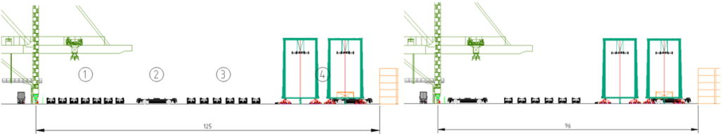 Figure 1: Typical cross section of AGV terminal with ASCs (left) vs. the proposed arrangement (right)
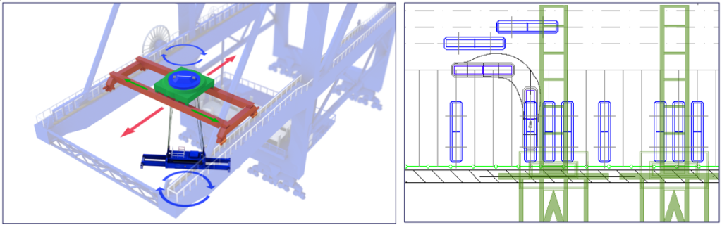
To accommodate this, the secondary / landside trolley needs two additional functionalities:
- Rotation of the container by 90 degrees.
- Sideways movement to reach the three transfer points dedicated to that quay crane.
Figure 2 shows a 3D impression of the secondary trolley. The image shows the sideways movement of the trolley, as well as the rotation. For more details on the proposed arrangement, reference is made the original article.
Simulation scenario
To evaluate the performance potential of the proposed narrow arrangement versus the original AGV arrangement, a detailed, dynamic simulation is conducted.
- The simulation is based on a fictional terminal, with the following characteristics:
- 1,200 meter quay with 12 quay cranes
- 31 stack modules with Automated Stacking Cranes (ASC) – 2 ASCs per block
- Yearly volume of 2.8 M TEU
- 30% transshipment / 70% import & export cargo
- Target QC productivity of 35 net containers per hour (gross around 32 bx/h).
A peak simulation is used for the evaluation. This means that in the simulation the terminal is working consistently at high workload. In this instance, this means:
- 12 cranes in operation as per Figure 3
- 10% of containers are (un)loaded in tandem by the main crane hoist, 20% of containers are (un)loaded in twin and remainder is (un)loaded in single operation
- 310 landside moves per hour (all truck moves, no rail)
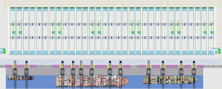 Figure 3: 2d view of the simulated terminal
Simulations are conducted for a range of lolo AGVs, starting from 48 AGVs (4 per quay crane) to 84 AGVs (7 per quay crane).
Simulation results
Figure 4 shows the average net QC performance for both scenarios. Based on extrapolation of the results, the standard AGV layout would required 74 AGVs in total (6.2 AGVs per QC) to reach the target of 35 net moves per hour. The narrow AGV layout can achieve the target with 70 AGVs (5.8 AGVs per QC).
What also can be observed is that with more AGVs, the QC performance is the same for both options. At this point, the AGVs are not the main bottleneck, but the QCs and ASC are the limiting factors.
When reducing the number of AGVs, the narrow AGV layout achieves a better performance. At this point the AGVs are the bottleneck in the system and as the narrow AGV layout benefits from shorter driving distances, a better performance is achieved.
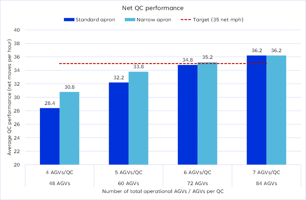 Figure 4: Average QC performance compared
Table 1 shows a number of key KPIs comparing both scenarios. The table shows some key differences between the two options at the target level performance of 35 net moves per hour.
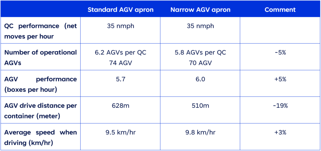 Table 1: Overview of main KPI
In the narrow AGV option, AGVs achieve 5% higher performance. This performance increase is a result of shorter drive distances. The driving distance per container is reduced by 19% (510 meter vs. 628 meter).
This shorter distance is achieved by the direct access to the QC transfer points, where as in the regular AGV layout, AGVs have to drive via the interchange lanes. In a dense cluster, this can be a tunnel of 3 to 4 cranes that the AGV needs to pass.
The distance reduction also directly translates into a reduction of energy consumption, allowing the AGV to operate longer on a battery charge.
What also can be observed is that the average driving speeds are slightly higher for the narrow apron design. This is caused by two main reasons:
- The narrow apron design does not require door turn moves by the AGV as the rotating spreader will take care of the door direction.
- The narrow apron design does not require any slow crab moves where as in the standard AGV, crab moves are used to access the QC transfer lane.
Concluding remarks.
The initial evaluation of the narrow apron design, already showed that the required apron “depth” to accommodate AGVs can be reduced from 125m to 96m. This space reduction translates into more than 10% extra storage capacity (or a smaller terminal footprint).
These simulations show that from a performance point of view, the narrow apron design can support at least similar, if not better, quay crane performance than the standard design (+5% in this specific example).
Another key outcome is that the driving distance per container is reduced by 19%. This translates in a considerable saving in energy consumption per container directly reducing OPEX as well as reduced requirement for charging (extra AGVs and chargers).
This article has been written by Jeroen Kats, Project Director at Portwise.