Decoupling impact versus driving distance
Today, I’d like to discuss a theme that keeps coming back in our planning work, and that is the (beneficial) effect of decoupling. With decoupling we mean the effect that one equipment type can operate in a (partially) independent way of another piece of equipment, where a terminal tractor (TT) has to wait for both an RTG and the QC, a straddle carrier waits for neither (although at the QC there can be some interference).
This waiting time is typically a large part of the TT or AGV (in the range of 40-60%), hence the “low” productivities of these machines.
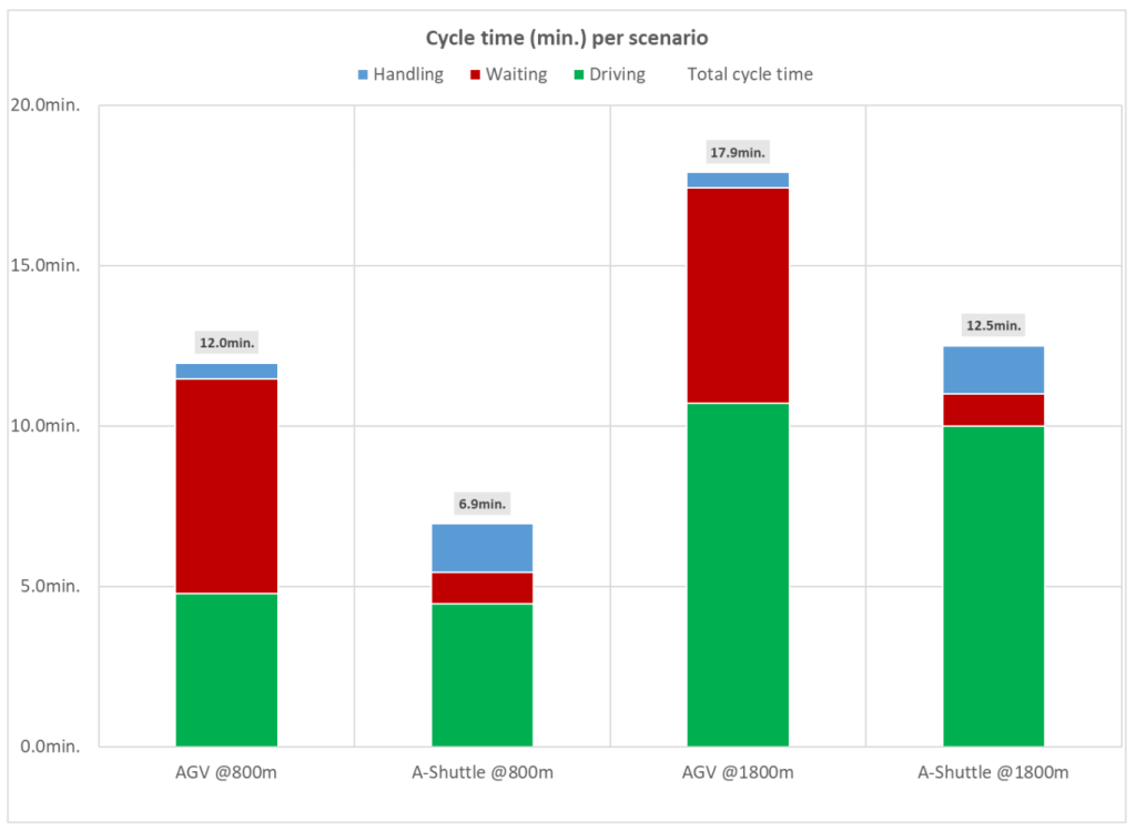
The positive effect of decoupling increases with the reduction in driving distance, as the portion of driving reduces with a decreasing distance. So in terminals with perpendicular ARMG’s (also: ASC’s), the driving distance from the stack interchange zones to the QC (or vice versa) is relatively short (typically between 600-800m): the effect of decoupling is large (see scenario 800m): the cycletime of an TT or AGV (driving + waiting) is about 12min. (of which only 5 minutes of driving, the remainder it’s standing still) and for the (automated) shuttle carrier it’s just short of 7min. (very limited waiting, but increased handling time for picking and dropping the container) (43% less). If however, the distances are longer (because the quay is further away, or there is significant % of transshipment), the effect reduces (scenario 1,800m). As a result the relative benefit of decoupling becomes less (only 30% remains). This because the waiting remains the same (in absolute terms) for the vehicles, but the driving more than doubles.

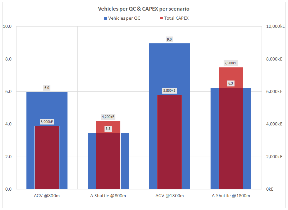
As equipment with decoupling capability is more expensive (to buy: CAPEX, to run: OPEX), the impact on CAPEX of driving distance needs to be considered. As can be seen in the 2nd graph (below), this can be quite substantial: CAPEX is almost equal in the case of short driving distances; where we need 6 AGV’s to get to a productivity of 30 bx/h and 3.5 automated shuttles), and 30% higher in the case of longer driving distances (where we need for 9 AGV’s and 6.3 Shuttles per QC).

This simple example emphasizes the importance of specific analysis for a specific case: the difference between handling systems can change based on the actual case at hand. For this purpose, Portwise always recommend to use dynamic simulation to analyse these effects, and come to educated decisions about these high impact (in terms of financials) aspects of a case.
About the author: Yvo Saanen is a seasoned container terminal consultant who has worked for over 25 years in the industry, assisting terminals across the globe in getting the most out of their facility, or planning a future proof terminal.